Forced quantum harmonic oscillator¶

Section author: Josh Izaac <josh@xanadu.ai>

Simulating the time-propagation of a Gaussian Hamiltonian using a continuous-variable (CV) quantum circuit is simple with SFOpenBoson. In this tutorial, we will walk through a simple example using the forced quantum harmonic oscillator.

Background¶

The Hamiltonian of the forced quantum harmonic oscillator is given by

\[\hat{H} = \frac{\p^2}{2m} + \frac{1}{2}m\omega^2 \q^2 - F\q\]

where

\(m\) is the mass of the oscillator,
\(\omega\) is the frequency of oscillation,
\(F\) is a time-independent external force.

Let’s define this Hamiltonian using OpenFermion, with \(m=\omega=1\) and \(F=2\):

>>> from openfermion.ops import QuadOperator
>>> from openfermion.utils import commutator, normal_ordered
>>> H = QuadOperator('q0 q0', 0.5) + QuadOperator('p0 p0', 0.5) - QuadOperator('q0', 2)

In the Heisenberg picture, the time-evolution of the \(\q\) and \(\p\) operators is given by:

\[\begin{split}& \frac{d}{dt}\q = \frac{i}{\hbar}[\hat{H}, \q] = \p\\ & \frac{d}{dt}\p = \frac{i}{\hbar}[\hat{H}, \q] = F-\q\end{split}\]

We can double check these using OpenFermion:

>>> (1j/2)*normal_ordered(commutator(H, QuadOperator('q0')), hbar=2)
1 [p0]
>>> (1j/2)*normal_ordered(commutator(H, QuadOperator('p0')), hbar=2)
2 [] + -1 [q0]

Assuming the oscillator has initial conditions \(\q(0)\) and \(\p(0)\), it is easy to solve this coupled set of linear differential analytically, giving the parametrised solution

\[\begin{split}&\q(t) = (\q(0)-F)\cos(t) + \p(0)\sin(t) + F\\ &\p(t) = (F-\q(0))\sin(t) + \p(0)\cos(t)\end{split}\]

Let’s now attempt to simulate these dynamics directly in Strawberry Fields, solely from the Hamiltonian we defined above.

Strawberry Fields simulation¶

To simulate the time-propagation of the forced oscillator in StrawberryFields, we also need to import the GaussianPropagation class from the SFOpenBoson plugin:

>>> import strawberryfields as sf
>>> from strawberryfields.ops import *
>>> from sfopenboson.ops import GaussianPropagation

GaussianPropagation accepts the following arguments:

operator: a bosonic Gaussian Hamiltonian, either in the form of a BosonOperator or QuadOperator.
t (float): the time propagation value. If not provided, default value is 1.
mode (str): By default, mode='local' and the Hamiltonian is assumed to apply to only the applied qumodes. For example, if QuadOperator('q0 p1') | (q[2], q[4]), then q0 acts on q[2], and p1 acts on q[4].

Alternatively, you can set mode='global', and the Hamiltonian is instead applied to the entire register by directly matching qumode numbers of the defined Hamiltonian; i.e., q0 is applied to q[0], p1 is applied to q[1], etc.

Let’s set up the one qumode quantum circuit, propagating the forced oscillator Hamiltonian H we defined in the previous section, starting from the initial location \((1,0.5)\) in phase space, for time \(t=1.43\):

>>> prog = sf.Program(1)
>>> with prog.context as q:
...     Xgate(1) | q[0]
...     Zgate(0.5) | q[0]
...     GaussianPropagation(H, 1.43) | q

Now, we can run this simulation using the Gaussian backend of Strawberry Fields, and output the location of the oscillator in phase space at time \(t=1.43\):

>>> eng = sf.Engine("gaussian")
>>> state = eng.run(prog).state
>>> state.means()
array([ 2.35472067,  1.06027036])

We compare this to the analytic solution,

\[\begin{split}&\braket{\q(1.43)} = (1-2)\cos(1.43) + 0.5\sin(1.43) + 2 = 2.35472,\\ &\braket{\p(1.43)} = (2-1)\sin(1.43) + 0.5\cos(1.43) = 1.06027,\end{split}\]

which is in good agreement with the Strawberry Fields result.

We can also print the CV gates applied by the engine, to see how our time-evolution operator \(e^{-i\hat{H}t/\hbar}\) got decomposed:

>>> eng.print_applied()
Xgate(1),       (reg[0])
Zgate(0.5),     (reg[0])
Rgate(-1.43),   (reg[0])
Xgate(1.719),   (reg[0])
Zgate(1.98),    (reg[0])

Plotting the phase-space time evolution¶

By looping over various values of \(t\), we can plot the phase space location of the oscillator for various values of \(t\).

Consider the following example:

eng = sf.Engine("gaussian")

t_vals = np.arange(0, 6, 0.02)
results = np.zeros([2, len(t_vals)])

for step, t in enumerate(t_vals):
        prog = sf.Program(1)

    with prog.context as q:
        Xgate(1) | q[0]
        Zgate(0.5) | q[0]
        GaussianPropagation(H, t) | q

    state = eng.run(prog).state
    eng.reset()
    results[:, step] = state.means()

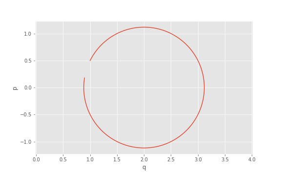
Here, we are looping over the same circuit as above for values of \(t\) within the domain \(0\leq t<6\), and storing the resulting expectation values \((\braket{\q(t)}, \braket{\p(t)})\) in the array results. We can plot this array in phase space:

>>> from matplotlib import pyplot as plt
>>> plt.plot(*results)